Workflow: How to use the serosurvey R package?
howto-reprex.RmdContext
Problem
- If we used an imperfect test to measure an outcome within a multi-stage sampling design survey, we need to incorporate the test uncertainty into the sampling design uncertainty.
Method details
survey:
- Sampling weights were included in a two-stage cluster sample without stratas. We estimated prevalence 95% confidence intervals using the “logit” method.
serology:
Here we applied a Bayesian method to estimate the posterior probability of seroprevalence for a test with unknown performance (Daniel B. Larremore et al. 2020).
As inputs we used the expanded point estimate number of positive tests and total population that resulted from the sampling weights adjusted seroprevalence estimation.
To maintain the sampling design uncertainty, we applied the same method for each estimated confidence interval.
Since test sensitivity and specificity were unknown, we used the reported number of true positives, false positives, true negatives and false negatives from a local test performance evaluation.
-
For this worlflow we used lab validation results from an example available in the
epiRpackage:?epiR::epi.tests- for sensitivity: Of 744 patients that were disease positive, 670 were test positive.
- for specificity: Of 842 patients that were disease negative, 640 were test negative.
Workflow details
In this reprex the survey design does not include any explicit strata. Include it if available in I.3.
The family of functions
serosvy_*_sample_posteriorto correct prevalence due to test performance require positive integers. This is adressed in II.2.1.We use
purrrandfurrrwithin afor-loopin II.2.2 to efficiently update prevalence posterior distributions for multiple prevalences.
Limitations
We do not apply a multiple subpopulation aproach for the inference of prevalence. This is currently available for a test with known performance (Daniel B Larremore et al. 2020).
This workflow is only applicable to categorical variables.
set.seedcould not control the variability generated by test correction functions.
I.1. Import data
-
datasurveyis the input dataframe - outcomes:
outcome_oneandoutcome_two - covariates:
covariate_01andcovariate_02
data(api)

datasurvey <- apiclus2 %>%
  mutate(survey_all="survey_all") %>%
  # conviniently create variables
  # to identify outcomes and covariates throughout the script
  mutate(outcome_one = awards, # this have the serology results
         outcome_two = cut(pct.resp,breaks = 2),
         covariate_01 = stype,
         covariate_02 = both,
         # two stage cluster samples
         primary_sampling_unit = dnum,
         secondary_sampling_unit = snum,
         # strata = census_tracts, (activate if available)
         sampling_weights = pw) %>%
  # recode factor leves to replicate serology results
  mutate(outcome_one=fct_recode(outcome_one,
                                "negative"="No","positive"="Yes")) %>%
  mutate(outcome_two=fct_recode(outcome_two,
                                "negative"="(50,100]","positive"="(-0.1,50]"))
I.2. Identify sets numerators and denominators
- Using
selectandcolnameswe create strings of covariates
# outcome
outcome_set00 <- datasurvey %>%
  select(outcome_one,
         outcome_two) %>%
  colnames()

# denominators
covariate_set01 <- datasurvey %>%
  select(covariate_01,
         #covariate_03,
         #covariate_04,
         covariate_02) %>%
  colnames()

# numerators within outcome
covariate_set02 <- datasurvey %>%
  select(#covariate_01,
         #covariate_03
         #covariate_04
         covariate_02) %>%
  colnames()
I.3. Create a srvyr survey design object
# define how to treat strata with only one census tract
options(survey.lonely.psu = "certainty")

# uu_clean_data %>% count(dnum, snum)

# create survey sampling design ---------------------------------

design <- datasurvey %>%

  # the outcome must have complete observations
  filter(!is.na(outcome_one)) %>%
  # all census tracts must contain sampling weights
  filter(!is.na(sampling_weights)) %>%

  as_survey_design(
    # 1 - primary and secondary sampling unit
    id=c(primary_sampling_unit, secondary_sampling_unit),
    # 2 - activate if available
    # strata = strata, #clusters need to be nested in the strata
    # 3- weights or expansion factors
    weights = sampling_weights
  )
I.4 Example: Single estimation
How to use
serosvy_proportionfor a single estimationHere we exchage the numerator and denominator
serosvy_proportion(design = design,
                   denominator = covariate_01,
                   numerator = outcome_one) %>%
  select(-ends_with("_low"),-ends_with("_upp"),
         -ends_with("_cv"),-ends_with("_deff"))
#> # A tibble: 6 x 12
#>   denominator denominator_lev~ numerator numerator_level  prop prop_se
#>   <chr>       <fct>            <chr>     <fct>           <dbl>   <dbl>
#> 1 covariate_~ E                outcome_~ negative        0.211  0.0482
#> 2 covariate_~ E                outcome_~ positive        0.789  0.0482
#> 3 covariate_~ H                outcome_~ negative        0.852  0.0872
#> 4 covariate_~ H                outcome_~ positive        0.148  0.0872
#> 5 covariate_~ M                outcome_~ negative        0.552  0.172
#> 6 covariate_~ M                outcome_~ positive        0.448  0.172
#> # ... with 6 more variables: total <dbl>, total_se <dbl>, total_den <dbl>,
#> #   raw_num <int>, raw_den <int>, raw_prop <dbl>

serosvy_proportion(design = design,
                   denominator = outcome_one,
                   numerator = covariate_01) %>%
  select(-ends_with("_low"),-ends_with("_upp"),
         -ends_with("_cv"),-ends_with("_deff"))
#> # A tibble: 6 x 12
#>   denominator denominator_lev~ numerator numerator_level   prop prop_se
#>   <chr>       <fct>            <chr>     <fct>            <dbl>   <dbl>
#> 1 outcome_one negative         covariat~ E               0.400   0.102
#> 2 outcome_one negative         covariat~ H               0.318   0.131
#> 3 outcome_one negative         covariat~ M               0.283   0.0783
#> 4 outcome_one positive         covariat~ E               0.840   0.0498
#> 5 outcome_one positive         covariat~ H               0.0311  0.0165
#> 6 outcome_one positive         covariat~ M               0.129   0.0435
#> # ... with 6 more variables: total <dbl>, total_se <dbl>, total_den <dbl>,
#> # raw_num <int>, raw_den <int>, raw_prop <dbl>II.1. Estimates: raw + weighted
outcome_01_pre <-
  # create a expanded grid of numerators and denominators
  #
  # set 01 of denominator-numerator
  #
  expand_grid(
    design=list(design),
    denominator=covariate_set01, # covariates
    numerator=outcome_set00 # outcomes
  ) %>%
  #
  # set 02 of denominator-numerator (e.g. within main outcome)
  #
  union_all(
    expand_grid(
      design=list(design),
      denominator=outcome_set00, # outcomes
      numerator=covariate_set02 # covariates
    )
  ) %>%
  #
  # create symbols (to be readed as arguments)
  #
  mutate(
    denominator=map(denominator,dplyr::sym),
    numerator=map(numerator,dplyr::sym)
  ) %>%
  #
  # estimate prevalence
  #
  mutate(output=pmap(.l = select(.,design,denominator,numerator),
                     .f = serosvy_proportion)) %>%
  #
  # show the outcome
  #
  select(-design,-denominator,-numerator) %>%
  unnest(cols = c(output)) #%>%

outcome_01_pre
#> # A tibble: 25 x 23
#>    denominator denominator_lev~ numerator numerator_level   prop prop_low
#>    <chr>       <fct>            <chr>     <fct>            <dbl>    <dbl>
#>  1 covariate_~ E                outcome_~ negative        0.211   0.130
#>  2 covariate_~ E                outcome_~ positive        0.789   0.675
#>  3 covariate_~ H                outcome_~ negative        0.852   0.564
#>  4 covariate_~ H                outcome_~ positive        0.148   0.0377
#>  5 covariate_~ M                outcome_~ negative        0.552   0.224
#>  6 covariate_~ M                outcome_~ positive        0.448   0.160
#>  7 covariate_~ E                outcome_~ positive        0.182   0.0499
#>  8 covariate_~ E                outcome_~ negative        0.818   0.515
#>  9 covariate_~ H                outcome_~ positive        0.0769  0.00876
#> 10 covariate_~ H                outcome_~ negative        0.923   0.560
#> # ... with 15 more rows, and 17 more variables: prop_upp <dbl>,
#> #   prop_cv <dbl>, prop_se <dbl>, total <dbl>, total_low <dbl>,
#> #   total_upp <dbl>, total_cv <dbl>, total_se <dbl>, total_deff <dbl>,
#> #   total_den <dbl>, total_den_low <dbl>, total_den_upp <dbl>,
#> #   raw_num <int>, raw_den <int>, raw_prop <dbl>, raw_prop_low <dbl>,
#> #   raw_prop_upp <dbl>
II.2. Add uncertain test performance
II.2.1 Filter serology results and add validation study results
-
Here we use:
Filter the rows with the results of the serology test:
outcome_oneRound population estimates to use positive integers in the next step
Add the results from the available validation study as columns
# _ 2. test performance ---------------------------------------------------

# __ filter + add values --------------------------------------------------

outcome_01_adj_pre <-
  outcome_01_pre %>%
  # only serological results
  filter(numerator=="outcome_one") %>%
  # only positives
  filter(numerator_level=="positive") %>%
  # round numbers are required
  mutate_at(.vars = vars(total,total_den,
                         total_low,total_den_low,
                         total_upp,total_den_upp),
            .funs = list("round"=round),digits = 0) %>%
  # unknown test local validation results
  # for sensitivity:
  # Of 744 patients that were disease positive, 670 were test positive.
  # for specificity:
  # Of 842 patients that were disease negative, 640 were test negative.
  # source: ?epiR::epi.tests
  mutate(
    true_positive = 670,
    false_negative = 74,
    false_positive = 202,
    true_negative = 640
  ) %>%
  rownames_to_column() %>%
  mutate(rowname=as.numeric(rowname))
II.2.2 Apply to all rows and extract the results
Here we use
purrrandfurrrwithin afor-loopto efficiently update prevalence posterior distributions for multiple prevalences.We apply the procedure to each point estimate and confidence interval
# 56-60sec por covariable
# 4GB RAM
# parallelized in 8 cores using purrr y furrr

plan(multisession, workers = availableCores())
tic()

out <- tibble()

for (i in 1:nrow(outcome_01_adj_pre)) {

  out <- outcome_01_adj_pre %>%

    slice(i) %>%

    # dot
    mutate(adj_dot_unk=future_pmap(
      .l = select(.,
                  positive_number_test=total_round,
                  total_number_test=total_den_round),
      .f = possibly(serosvy_unknown_sample_posterior,otherwise = NA_real_),
      true_positive = true_positive,
      false_negative = false_negative,
      false_positive = false_positive,
      true_negative = true_negative)) %>%
    serosvy_extract_posterior(variable = adj_dot_unk) %>%

    # low
    mutate(adj_low_unk=future_pmap(
      .l = select(.,
                  positive_number_test=total_low_round,
                  total_number_test=total_den_low_round),
      .f = possibly(serosvy_unknown_sample_posterior,otherwise = NA_real_),
      true_positive = true_positive,
      false_negative = false_negative,
      false_positive = false_positive,
      true_negative = true_negative)) %>%
    serosvy_extract_posterior(variable = adj_low_unk) %>%

    # upp
    mutate(adj_upp_unk=future_pmap(
      .l = select(.,
                  positive_number_test=total_upp_round,
                  total_number_test=total_den_upp_round),
      .f = possibly(serosvy_unknown_sample_posterior,otherwise = NA_real_),
      true_positive = true_positive,
      false_negative = false_negative,
      false_positive = false_positive,
      true_negative = true_negative)) %>%
    serosvy_extract_posterior(variable = adj_upp_unk) %>%

    # union all outputs
    union_all(out)

  # activate to print the progress! (recommended)
  # out %>% print() #%>%

  # # known test
    # mutate(adj_dot_kno=future_pmap(
    #   .l = select(.,
    #               positive_number_test=total_round,
    #               total_number_test=total_den_round),
    #   .f = possibly(serosvy_known_sample_posterior,otherwise = NA_real_),
    #   sensitivity=0.999,
    #   specificity=0.960))

}

toc()
#> 573.72 sec elapsed

outcome_01_adj <- out  %>%
  mutate(rowname=as.numeric(rowname)) %>%
  arrange(rowname) %>%
  select(-rowname)
II.3. Create output format
Here we join all the results to the original dataset
We also create
unite*_columns summarizing the results
outcome_01_adj_tbl <-
  # start from original dataset
  outcome_01_pre %>%
  # only positives
  filter(numerator_level=="positive"|denominator_level=="positive") %>%
  # left join with db with test performance update
  left_join(outcome_01_adj) %>%
  # naniar::miss_var_summary() %>%
  # avallecam::print_inf() %>%

  # apply format
  unite_dotwhiskers(variable_dot = raw_prop,
                    variable_low = raw_prop_low,
                    variable_upp = raw_prop_upp,
                    digits_dot = 2,
                    digits_low = 1,
                    digits_upp = 2) %>%
  unite_dotwhiskers(variable_dot = prop,
                    variable_low = prop_low,
                    variable_upp = prop_upp,
                    digits_dot = 2,
                    digits_low = 1,
                    digits_upp = 2) %>%
  unite_dotwhiskers(variable_dot = adj_dot_unk_p50,
                    variable_low = adj_low_unk_p50,
                    variable_upp = adj_upp_unk_p50,
                    digits_dot = 3,
                    digits_low = 2,
                    digits_upp = 3)
II.4. Evaluate output
-
Take a quick look to the output:
-
raw_or_unadjusted_prevcrude or raw prevalence -
sampling_weighted_prevsampling weights adjusted prevalence -
sampling_and_test_prevsampling weights and test performance adjusted prevalence
-
outcome_01_adj_tbl %>%
  select(1:4,raw_num,raw_den,
         starts_with("unite1_"),
         prop_cv) %>%
  rename("raw_or_unadjusted_prev"=unite1_raw_prop,
         "sampling_weighted_prev"=unite1_prop,
         "sampling_and_test_prev"=unite1_adj_dot_unk_p50) %>%
  mutate_if(.predicate = is.numeric,.funs = ~round(.x,2)) %>%
  #   DT::datatable()
  knitr::kable() %>%
kableExtra::kable_styling(bootstrap_options = "striped", full_width = F)| denominator | denominator_level | numerator | numerator_level | raw_num | raw_den | raw_or_unadjusted_prev | sampling_weighted_prev | sampling_and_test_prev | prop_cv |
|---|---|---|---|---|---|---|---|---|---|
| covariate_01 | E | outcome_one | positive | 63 | 83 | 75.9 (65.3 - 84.6) | 78.9 ( 67.5 - 87) | 83.150 (65.89 - 95.5) | 0.06 |
| covariate_01 | H | outcome_one | positive | 5 | 20 | 25.0 ( 8.7 - 49.1) | 14.8 ( 3.8 - 44) | 0.425 ( 0.28 - 29.9) | 0.59 |
| covariate_01 | M | outcome_one | positive | 15 | 23 | 65.2 (42.7 - 83.6) | 44.8 ( 16.0 - 78) | 31.506 ( 0.40 - 81.1) | 0.38 |
| covariate_01 | E | outcome_two | positive | 5 | 83 | 6.0 ( 2.0 - 13.5) | 18.2 ( 5.0 - 49) | NA | 0.58 |
| covariate_01 | H | outcome_two | positive | 1 | 20 | 5.0 ( 0.1 - 24.9) | 7.7 ( 0.9 - 44) | NA | 0.96 |
| covariate_02 | Yes | outcome_one | positive | 83 | 89 | 93.3 (85.9 - 97.5) | 96.7 ( 88.2 - 99) | 99.901 (96.99 - 100.0) | 0.02 |
| covariate_02 | No | outcome_two | positive | 3 | 37 | 8.1 ( 1.7 - 21.9) | 21.8 ( 6.7 - 52) | NA | 0.51 |
| covariate_02 | Yes | outcome_two | positive | 3 | 89 | 3.4 ( 0.7 - 9.5) | 9.1 ( 2.1 - 32) | NA | 0.68 |
| outcome_one | positive | covariate_02 | Yes | 83 | 83 | 100.0 (95.7 - 100.0) | 100.0 (100.0 - 100) | NA | 0.00 |
| outcome_two | positive | covariate_02 | No | 3 | 6 | 50.0 (11.8 - 88.2) | 54.9 ( 29.4 - 78) | NA | 0.15 |
| outcome_two | positive | covariate_02 | Yes | 3 | 6 | 50.0 (11.8 - 88.2) | 45.1 ( 21.9 - 71) | NA | 0.19 |
II.5. Output figure
- Make a quick plot using a custom created function
outcome_01_adj_tbl %>%
  filter(str_detect(numerator,"outcome")) %>%
  ggplot_prevalence(
    denominator_level = denominator_level,
    numerator = numerator,
    proportion = prop,
    proportion_upp = prop_upp,
    proportion_low = prop_low) +
  # theme(axis.text.x = element_text(angle = 0, vjust = 0, hjust=0)) +
  scale_y_continuous(
    labels = scales::percent_format(accuracy = 1),
    breaks = scales::pretty_breaks(n = 5)) +
  # coord_flip() +
  facet_wrap(denominator~.,scales = "free") +
  # facet_grid(denominator~.,scales = "free_y") +
  colorspace::scale_color_discrete_qualitative() +
  labs(title = "Prevalence of numerators across denominators",
       y = "Prevalence",x = "")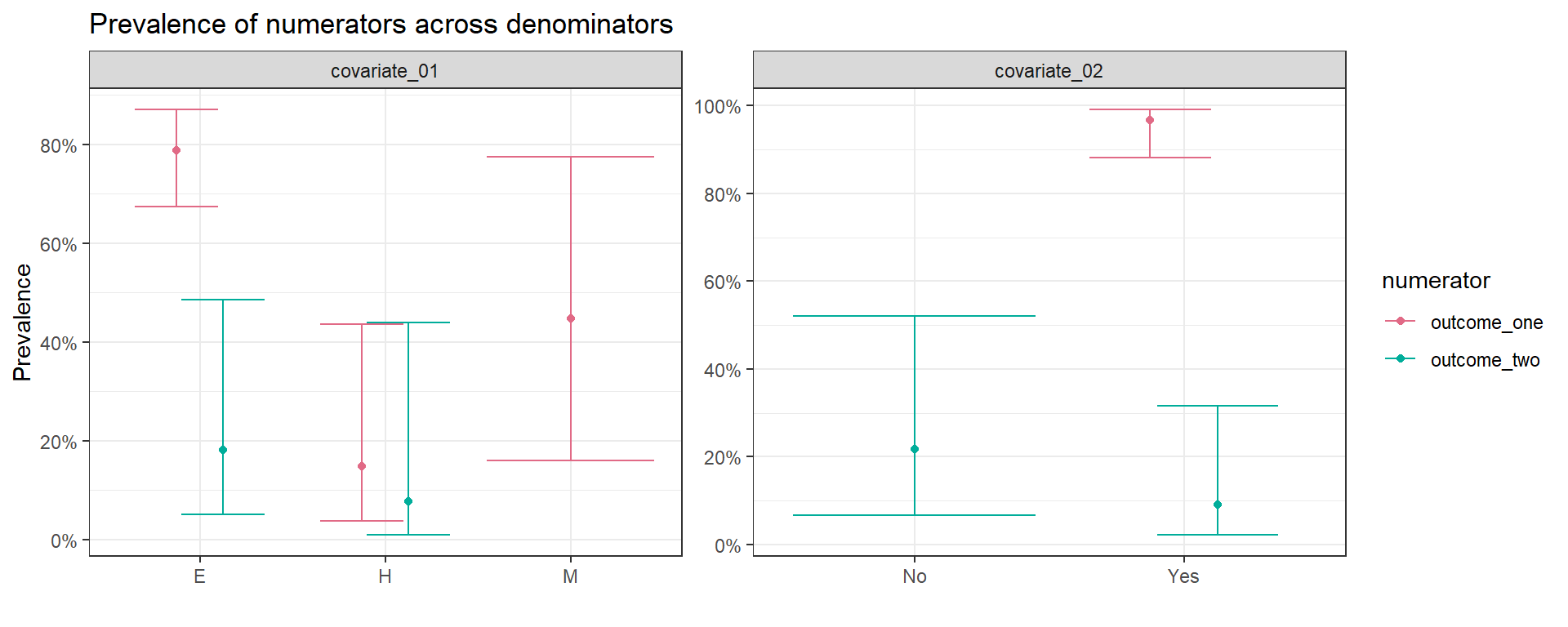
Reference
Larremore, Daniel B, Bailey K Fosdick, Kate M Bubar, Sam Zhang, Stephen M Kissler, C. Jessica E. Metcalf, Caroline Buckee, and Yonatan Grad. 2020. “Estimating SARS-CoV-2 Seroprevalence and Epidemiological Parameters with Uncertainty from Serological Surveys.” medRxiv, April. https://doi.org/10.1101/2020.04.15.20067066.
Larremore, Daniel B., Bailey K. Fosdick, Sam Zhang, and Yonatan H. Grad. 2020. “Jointly Modeling Prevalence, Sensitivity and Specificity for Optimal Sample Allocation.” bioRxiv, May. https://doi.org/10.1101/2020.05.23.112649.